Magic Behind Constructing A Decision Tree

Before we get started I need to clarify something. Theoretical decision trees can have two or more branches protruding from a single node.

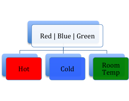
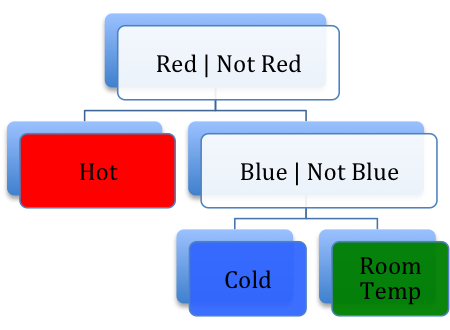
However, this can be computationally expensive so most implementations of decision trees only allow binary splits.

Recall our example problem – Bill is a user on our online dating site and we want to build a decision tree that predicts whether he would message a certain woman. (If so, we say that she’s “date-worthy”). Suppose we have the following ten samples of women who Bill has viewed and messaged.

ID	Distance	Hair	Income	Height	BillMessagedHer?
1	5	Blonde	100	5’6	TRUE
2	20	Blonde	50	5’11	FALSE
3	100	Red	20	5’2	FALSE
4	40	Brown	45	6’0	FALSE
5	250	Brown	200	5’5	TRUE
6	5	Blonde	20	6’1	FALSE
7	15	Brown	0	4’11	FALSE
8	20	Black	80	5’3	TRUE
9	70	Brown	15	5’3	FALSE
10	30	Brown	85	5’8	FALSE

Given these 10 training samples, what’s the best split point we can choose to separate our data? Let’s analyze a couple of arbitrary splits.

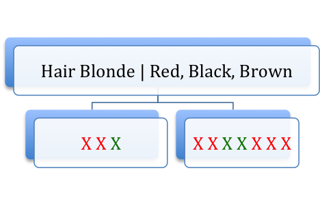
Here, green Xs signify women who Bill messaged and red Xs signify women who Bill didn’t message. Out of 3 women with blonde hair, Bill messaged 1 of them and out of 7 women without blonde hair, Bill messaged 2 of them.

Out of 6 women 5’6 and shorter Bill messaged 3 of them, and out of 4 women taller than 5’6 Bill messaged 0 of them.

It appears Bill cares about womens’ height more than their hair color. Maybe Bill is 5’7 and only dates women shorter than him. Whatever the case, we think that split #2 is a better predictor of women who Bill would message.

The above comparison was pretty intuitive but that isn’t always the case. Suppose we compare these two splits:

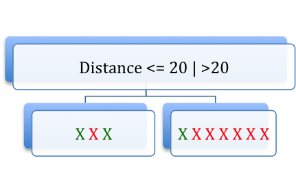
Which is the better split? This is a subjective question. In practice, people use different metrics for evaluating splits. The most commonly used metric is Information Gain. Another commonly used metric is Gini Impurity, and since it’s easier to explain, let’s use it.

Gini Impurity measures the disorder of a set of elements. It is calculated as the probability of mislabeling an element assuming that the element is randomly labeled according the the distribution of all the classes in the set.

Example: Suppose we have a set with 6 elements: {red, red, blue, blue, blue, blue}. (The classes of this set are red and blue). We select an element at random. Then we randomly label it according to the distribution of classes in the set. This would be equivalent to labeling the selected element by rolling a 6 sided die with 4 blue sides and 2 red sides. The probability that we misclassify the element is equal to the probability that we select a red element times the probability that we label it blue plus the probability that we select a blue element times the probability that we label it red. This is

2/6 * 4/6 + 4/6 * 2/6 = 16/36.

A few points before we move on. If all the elements in a set are identical, the Gini Impurity is 0. If we have two classes of elements, our max Gini Impurity occurs when there is an equal number of elements from each class in the set. In this case the Gini Impurity is 1/2. Gini Impurity generalizes for more than 2 classes, and the max Gini Impurity approaches 1 as the number of classes approaches infinity.

Now suppose we have a set {red, red, blue, blue, blue, blue}. We consider a split {red blue blue blue} {red blue}. We can measure the goodness of this split by averaging the Gini Impurity of the leaves, weighted by the number of elements in each leaf and compare that number to the Gini Impurity in the root.

The Gini Impurity in the root was 16/36 = 0.444. The weighted average of the Gini Impurity in the leaves is roughly 0.417 So this split reduced our Impurity by about 0.027.

Now we have a method to quantify the goodness of a split, but how do we know what splits to test? Implementations differ here. Ideally, we’d like to test all possible splits but this isn’t always practical. There are typically 4 types of feature vectors:

Boolean – True or False

Numerical – In our example Distance and Income are numerical features.

Factors – Loosely speaking, factors are variables that have a limited number of possible values. Factors can be subdivided into two categories

Unordered Factors – This would be like hair color. In our example we had Blonde, Red, Brown, and Black and for our purposes it doesn’t do us any good to try to order these. Ordered Factors – Height. Okay, this one’s borderline numerical but let’s just assume that our website only allows users to select heights between 4’ and 7’ with 1 inch intervals. The important thing to recognize is that we have a finite set of possible values where order matters. First let’s look at our vector of Incomes.

Income	BillMessagedHer?
100	TRUE
50	FALSE
20	FALSE
45	FALSE
200	TRUE
20	FALSE
0	FALSE
80	TRUE
15	FALSE
85	FALSE

How might we write a program to test various splits? It’s easy to get creative here but a simple program would just order the incomes and try the midpoint of each interval. The Gini Impurity reduction for each split would be calculated and the split with the best reduction would be kept.

Next up, unordered factors. What splits would we test on the possible hair colors? In this case all of them,

{Blonde} vs {Red or Brown or Black}
{Blonde or Red} vs {Brown or Black}
{Blonde or Brown} vs {Red or Black}
{Blonde or Black} vs {Red or Brown}
{Blonde or Red or Brown} vs {Black}
{Blonde or Red or Black} vs {Brown}
{Blonde or Black or Brown} vs {Red}

That’s seven unique splits. Here’s the catch – as the number of classes grows, the number of unique splits blows up. Implementations for handling this differ, but one common method is to simply throw an error if there are too many unordered factor classes in the dataset.

Lastly, ordered factors. This is handled in the obvious way. Test all the possible splits without mixing up the order of the factors. If your factors are {Strongly Disagree, Disagree, Agree, Strongly Agree} your splits would be

{Strongly Disagree} vs {Disagree, Agree, Strongly Agree}
{Strongly Disagree, Disagree} vs {Agree, Strongly Agree}
{Strongly Disagree, Disagree, Agree} vs {Strongly Agree}

Now we know what splits to test and how to compare them. We can grow our tree one level out from the root node!

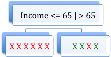
In what direction should we grow our tree?

Depth First…

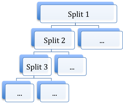
or Breadth First?

Frankly, it doesn’t matter. Let’s suppose we grow our tree depth first.

The algorithm for growing a decision tree is an example of recursive partitioning. Each node in the tree is grown using the same set of rules as its parent node and the data in the parent node gets partitioned into its child nodes. How do we know when to stop? Ahh, good question!

Clearly, if all of the elements in a node are of the same class it doesn’t do us much good to add another split. Doing so would usually decrease the predictive power of our model. This is known as overfitting. Naturally, this brings up the question, “What if we have a node with 50 elements of the same class and 1 element of a different class?” Hopefully you see where this is going. You, as the omniscient data scientist get to be creative with the rules for termination. Most implementations of decision trees provide a number of parameters for this.

(Special Thanks to Jesse Furmanek for correcting a calculation error in this post.)